DRAM - Delayed Rejection Adaptive Metropolis

This web page accompanies the article: H. Haario, M. Laine, A. Mira and E. Saksman, 2006. DRAM: Efficient adaptive MCMC, Statistics and Computing 16, pp. 339-354. (doi:10.1007/s11222-006-9438-0). Below, you find some computer experiment using Matlab. More general MCMC Matlab toolbox is available here.

DRAM is a combination of two ideas for improving the efficiency of Metropolis-Hastings type Markov chain Monte Carlo (MCMC) algorithms, Delayed Rejection and Adaptive Metropolis. This page explains the basic ideas behind DRAM and provides examples and Matlab code for the computations. Familiarity with MCMC methods in general is assumed, however.

Random walk Metropolis-Hasting algorithm with Gaussian proposal distribution is useful in simulating from the posterior distribution in many Bayesian data analysis situations. For example, in large class of nonlinear models we can write the model as

In order the chain to be efficient, the proposal covariance must somehow be tuned to the shape and size of the target distribution. This is important in highly nonlinear situations, when there are correlation between the components of the posterior, or when the dimension of the parameter is high. The problem of adapting the proposal distribution using the chain simulated so far is that when the accepted values depend on the history of the chain, it is no longer Markovian and standard convergence results do not apply. One solution is to use adaptation only for the burn-in period and discard the part of the chain where adaptation has been used. In that respect, the adaptation can be tough as automatic burn-in. The idea of diminishing adaptation is that when adaptation works well, its effect gets smaller and we might be able to prove the ergodicity properties of the chain even when adaptation is used throughout the whole simulation. This is the ideology behind AM adaptation. On the other hand, the DR method allows the use of the the current rejected values without losing the Markovian property and thus allows to adapt locally to the current location of the target distribution.

AM - Adaptive Metropolis

In Adaptive Metropolis, (Haario, et al. 2001) the covariance matrix of the Gaussian proposal distribution is adapted on the fly using the past chain. This adaptation destroys the Markovian property of the chain, however, it can be shown that the ergodicity properties of the generated sample remain. How well this works on finite samples and on high dimension is not obvious and must be verified by simulations.

Starting from initial covariance C₀, the target covariance is updated at given intervals from the chain generated so far.

DR

There is a way to make use of several tries after rejecting a value by using different proposals and keep the reversibility of the chain. Delayed rejection method (DR) (Mira, 2001a) works in the following way. Upon rejection a proposed candidate point, instead of advancing time and retaining the same position, a second stage move is proposed. The acceptance probability of the second stage candidate is computed so that reversibility of the Markov chain relative to the distribution of interest is preserved. The process of delaying rejection can be iterated for a fixed or random number of stages. The higher stage proposals are allowed to depend on the candidates so far proposed and rejected. Thus DR allows partial local adaptation of the proposal within each time step of the Markov chain still retaining the Markovian property and reversibility.

The first stage acceptance probability in DR is the standard MH acceptance and it can be written as

The smaller overall rejection rate of DR guarantees smaller asymptotic variance of the estimates based on the chain. The DR chain can be shown to be asymptotically more efficient that MH chain in the sense of Peskun ordering (Mira, 2001a). It should also be noted that DR in itself can be applied to much larger classes of problems than those described here.

DRAM

To be able to adapt the proposal at all you need some accepted points to start with. If we combine AM and DR we get method called DRAM (Haario, et al. 2006). We use different proposals in DR manner and adapt them as in AM. Many different implementations of the idea are possible. We demonstrate one quite straight forward possibility. One "master" proposal is tried first. After rejection, a try with modified version of the first proposal is done according to DR. Second proposal can be one with a smaller covariance, or with different orientation of the principal axes. The master proposal is adapted using the chain generated so far, and the second stage proposal follows the adaptation in obvious manner. In the examples, and in the dramrun Matlab function, the second stage is just a scaled down version of the first stage proposal that itself is adapted according to AM.

DRAM is illustrated in the following four examples. Matlab code for the first 3 examples are given at the end of this page.

Example 1 - banana shaped distribution

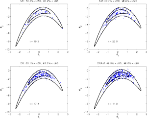
Here is a simple computer experiment to demonstrate all of the four combinations of the methods. Plain Metropolis-Hastings (MH), Delayed Rejection (DR), Adaptive Metropolis (AM), and DRAM. We start with 2 dimensional Gaussian distribution with unit variances and the correlation between the components equal to ρ (=0.9 in the example below). Then the Gaussian coordinates x₁ and x₂ are twisted to produce more nonlinear target. The twisting is done with equations

Fig. 1 2-d plots of the chain for the four methods. Contours give correct 50% and 95% regions. Percentages in the title show how many points lie inside the regions. Click the plot to enlarge.

We use Gaussian proposal with identity matrix as the initial proposal covariance. Chain of length 1000 is generated with each of the methods HM, DR, AM and DRAM. The mixing of the chain is studied by counting the number of point that are inside the 50% and 95% probability regions. As we generate only 1000 points, the observed percentages will vary from simulation to simulation, but we can see that all the methods are working correctly as expected. The initial proposal is not optimal for the plain MH and the acceptance ratio stays at about 10%. In addition, the chain does not have enough time to mix properly. DR without adaptation but with smaller 2^nd proposal makes the chain to accept more points, which helps the mixing, the acceptance ratio being about 30%. Both AM and DRAM make the chain to mix more quickly, due adaptation, and we see that also more distant points are visited. The covariance shrink factor for DR proposal is 2².

Number τ in the plots is the integrated autocorrelation time, giving the estimated increase of the asymptotic variance of the chain based estimates compared to an i.i.d. sample (Sokal, 1998). Number τ also varies from run to run, in general DRAM being the most efficient. Result τ = 11.0 here for DRAM means approximately that if using every 11. points from the chain, the sample behaves like an i.i.d. sample from the target distribution.

Example 2 - 20 d Gaussian with positivity

In this example the target is constructed from a 20 dimensional Gaussian distribution with singular values of the covariance matrix diminishing linearly from 10 to 1, thus the condition number of the covariance matrix is 10. The direction of the first principal axis is chosen to be [1,1,....,1]'. In addition, the density is centered at the origin and a positivity constraint is posed. The positivity is achieved simply by rejecting proposed new values when any of the coordinates is negative. Upon a reject, a new DR try with a smaller proposal can be made, however.

Fig. 2 First 3 components 20-d Gaussian target with positivity constraint, every 500. point of 500 000 iterations are shown. Click the plot to enlarge.

The initial proposal is again a Gaussian with identity matrix as the covariance. Rejecting negative values is computationally cheap, because likelihood needs not to be evaluated, but it causes the chain to stay at the current position, which increases the autocorrelation of the chain. After rejection, a new DR try is done with proposal covariance shrink factor 30². In fact, in the case of rejecting a value due to being outside the prior bounds, one could make a few extra tries with even smaller proposals to eventually get a new value accepted. This is not implemented in the code provided, however.

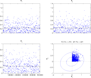A very large number of iterations is needed to get the chain to mix properly. The picture shows a plot of three first columns of the 20 dimensional chain. Fourth plot is 2d cloud of the first 2 coordinates, along with correct 50% and 95% contours. We are in a region that has volume of only 2^-20 times the distribution without the positivity restriction. This a very hard target to make to work efficiently with plain MH. DRAM seems to handle this situation correctly.

Example 3 - reaction kinetics

In this example the target is defined using a likelihood function with i.d.d. Gaussian errors in the observations. We consider a simple chemical reaction A<->B, where a component A goes to B in a reversible manner, with reaction rate coefficients k₁ and k₂. The dynamics are given by the ODE system:

Fig. 3 Data and lsq estimate for the A<->B example Click the plot to enlarge.

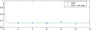Synthetic data is created for parameter values k₁ = 2, k₂ = 4 at time points t = 2,4,6,8,10. Zero mean Gaussian noise with standard deviation of size 0.01 is added. For the prior we set a broad Gaussian distribution with center point at (2,4) and standard deviation equal to 200 for both parameters.

Fig. 4 Plain Metropolis-Hastings chain Click the plot to enlarge.

With plain Metropolis-Hastings algorithm, the initial proposal is too small and the chain does not mix well. The orientation of the proposal is right however and almost all of the proposed points are accepted. High correlation between the parameters is visible.

Fig. 5 Adaptive Metropolis chain Click the plot to enlarge.

When we adapt the proposal the situation gets better. However some good accepted values are needed to get the adaptation work. Even in the simple 2-d situation it is possible for the adaptation to get lost when the adaptation is based in a too small sample. Some protection is needed in case the sample covariance matrix becomes singular. This can be achieved by adding small numbers to the diagonal of the sample covariance.

Fig. 6 DRAM chain Click the plot to enlarge.

In the DRAM chain, extra DR tries with a smaller proposal covariance makes the chain behave more robustly, as there are more points to adapt from right from the beginning.

In such a low dimensional situation, the chain typically is not sensitive with respect to the choice of the non-adaptation period, once the adaptation has properly started. However, if we have to start with a poor initial proposal, which might not produce accepted points at the very beginning. Here the initial period and also the adaptation interval is 100, and we are not able to to produce run where DRAM would fail.

Example 4 - algae kinetics

Fig. 7 Simplified example of algae dynamics in a lake Click the plot to enlarge.

This is a simplified lake algae dynamics model. Consider phytoplankton A, zooplankton Z and nutrition P (eg. phosphorus) available for A in the water. The system is affected by the water outflow/inflow Q, incoming phosphorus load P_in and temperature T. It is described as a simple predator - pray dynamics between A and Z. The growth of A is limited by the availability of P and it depends on the water temperature T. The inflow/outflow Q affects both A and P, but not Z. We use the following equations

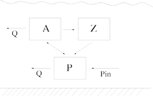The parameters to be estimated are

μmax	maximum growth rate for A at 20 °C
k	half saturation constant for the P demand of A
α	the filtration rate for grazing of Z
θ	temperature coefficient for A
ρa	non predatory loss of A
ρz	dying term for Z

We have observations of the state variables A, Z and P and time series data of the control variables Q, T and P_in.

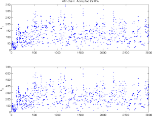
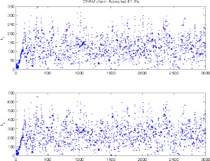
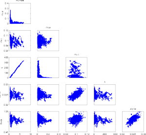
There are several things to be aware of when estimating this type of models. Firstly, we have to careful with the numerical behaviour of the solvers. During the simulation of the chain, we can get to be in regions of the posterior where the ODE system becomes extremely stiff, for example. Secondly, as some of the parameters are likely to be highly correlated and unidentified by the data, the approaches relying on linearizations of the model might not get realistic approximations of the uncertainties. Even when we use MCMC there might be problems in the convergence of the chain, as seen below.

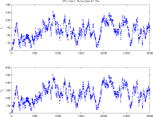
DRAM is useful in situations where the parameters are not very well identified by the data. As in the previous example it can happen that the posterior distributions are "infinite" to some directions. However, in higher dimensional situations this is not always clear in advance. Chain generated with fixed proposal can show very stable behaviour for a long time in a local mode of the posterior, before starting to explore the whole posterior.

Fig. 8 MH chain for the algae example. Click the plot to enlarge.

We generate a chain of length 10 000. Again we start from the parameters obtained by least squares minimization, and initial proposal is constructed from approximate Hessian matrix of the local sum-of-squares surface around the optimum.

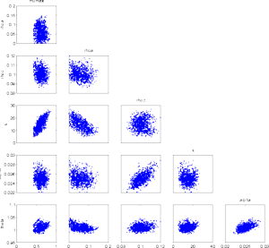At first, at least looking at the 2 d marginal chains, it seems that the chain has converged and has provided a nice sample from the posterior. It can be dangerous to rely on too short simulation when the dimensionality of the parameter is high or the parameters are correlated.

Fig. 9 Dram chain for the algae example showing the unidentifiability of some of the parameters. Click the plot to enlarge.

A DRAM run shows the problem. The 2d plots while looking more "unfinished" than that of the MH run, reveal the fact that the parameters k and μ^max do not identify at all. A large half saturation constant k can be compensated with large maximum growth rate. The plots of the generated chain, even if not fully converged, can give advise to model simplification or re-parametrization. The remedy is to gather more data, make a new experiment, if possible, with more variable algae concentrations, or provide prior information for unidentified parameters, or re-parametrizize the model.

Code

Computer code (Matlab 6.x) for the first three examples above are in a zip file dramcode.zip. No additional toolboxes are needed to run the code. Some utility functions for statistical computations are provided. The main functions and script included are the following.

dramrun.m

Matlab function for a dram MCMC run. The user provides her own Matlab function to calculate the "sum-of-squares" function for the likelihood part, eg. a function that calculates minus twice the log likelihood, -2log(p(θ;data)). Optionally a prior "sum-of-squares" function can also be given, returning -2log(p(θ)). If not given, the default priorfun returns always 0. See help dramrun for more details.

bananatest.m

Matlab commands to run and produce the plots of the banana example 1.

normaltest.m

Matlab command to run the Gaussian distribution with positivity requirement example 2.

ABrun.m

Matlab commands to run the chemical reaction example 3.

/utils

Subdirectory for some utility functions needed in the calculations.

References

H. Haario, M. Laine, A. Mira and E. Saksman, 2006. DRAM: Efficient adaptive MCMC, Statistics and Computing 16, pp. 339-354. (doi:10.1007/s11222-006-9438-0)

H. Haario, E. Saksman and J. Tamminen, 2001. An adaptive Metropolis algorithm Bernoulli 7, pp. 223-242.

L. Tierney and A. Mira, 1999. Some adaptive Monte Carlo methods for Bayesian inference. Statistics in Medicine, 18, pp. 2507-2515.

A. Mira, 2001a. On Metropolis-Hastings algorithm with delayed rejection Metron, Vol. LIX, 3-4, pp. 231-241.

P. J. Green and A. Mira, 2001b. Delayed rejection in reversible jump Metropolis-Hastings. Biometrika, Vol. 88, pp. 1035-1053.

A. D. Sokal, 1998. Monte Carlo methods in statistical mechanics: foundations and new algorithms. Cours de Troisième Cycle de la Physique en Suisse Romande, Lausanne.

A. G. Gelman, G. O. Roberts and W. R. Gilks, 1996. Efficient Metropolis jumping rules, Bayesian Statistics V, pp. 599-608 (eds J.M. Bernardo, et al.). Oxford University press.