EPPES parameter estimation example using Lorenz 95

This example demonstrates EPPES method using so called stochastic Lorenz 95 system [Wilks, 2005]. It is a Lorenz 95 system with added fast state variables whose effect is parameterized in the simpler forecast model. Here we estimate these parameters using EPPES. See the EPPES article [Laine, 2011] for details. This code is a slightly simplified version of the example in Section 4 of the paper.

Laine, et al.: Ensemble prediction and parameter estimation system: the method, Q. J. R. Meteorol. Soc., 2011, doi:10.1002/qj.922.

First, we load the truth system used as observations. The true states are generated with the full system using short integration time step and including the fast state variables, also. For estimation of the closure parameters of the simpler forecast model some independent random noise (with std sigma_a) is later added to these error free states.

T10 = load('T10.mat')

truth = T10.truth; % true states
aint  = T10.aint;  % analysis intervall
dt    = T10.dt;    % integration time step

T10 = 

    truth: [301x360 double]
     aint: 0.4
       dt: 0.0025

The forecast model function is obtained by evaluating the numerical solution of the L95 ode system at given time points and initial values at the start. The modified Lorenz 95 ode system is defined in file the l95ode.m.

l95fun = @(time,s0,params) deval(ode45(@l95ode,time,s0(:),[],params),time);

The standard deviations for analysis and initial perturbations.

sigma_a  = 0.05;
sigma_ip = 0.1;

Forecast model settings.

params.F       = 10;
params.sigma_e = 0;
params.phi     = 0.0;
params.gupars  = [0.0 0.2]; % initial parameter values
params.gufun   = @(x,p) polyval(p,x);
params.eta     = zeros(50,1);
fc_range       = 3;  % how long ahead do we forecast

nens = 50;  % ensemble size
npar = length(params.gupars); % number of parameters

Initial values for hyperprior parameters.

mu  = params.gupars(:); % initial prior mean
tau = 100*diag([1;1].^2); % accuracy of mu
sig = 0.1*diag([1;1].^2); % initial prior covariance
n0  = 1;                  % accuracy of sig
nmax = 10;                % maximum n0

Define number of EPPES iterations, and allocate memory for saving the intermediate results,

niter      = size(truth,1)-fc_range-1;
niter      = 30; % use a smaller number of iterations for faster illustration
parsall    = zeros(niter,nens,npar);
weightsall = zeros(niter,nens);
muall      = zeros(niter,npar);
sigall     = zeros(niter,npar,npar);

disp('running eppes, this will take some time ...')

running eppes, this will take some time ...

The simulation loop.

figure(1);clf
for iiter=1:niter

  time = (iiter-1)*aint:dt:(iiter+fc_range-1)*aint;
  a = truth(iiter,1:40);
  a = a + sigma_a*randn(size(a));  % analysis = truth + noise

  pars_prop = mvnorr(nens,mu,sig);  % proposed parameters from N(mu,sig)

  % launch the ensemble
  for j=1:nens
    s0 = a + sigma_ip*randn(size(a));       % initial value
    params.gupars = pars_prop(j,:);         % forecast model parameters
    sens(:,:,j) = l95fun(time,s0,params)';  % run the forecast model
    smod = sens(aint/dt:aint/dt:end,:,:);   % model response at data points
  end

  % sum of squares for ensemble members is calculated in function ens_ss_l95.m
  ss = ens_ss_l95(smod,truth(iiter+1:iiter+fc_range,1:40));
  % calculating weights and resampling
  w = exp(-0.5*(ss(:)));
  w = w/sum(w);
  pars_new = resample(pars_prop,w);

  % update the parameters
  [mu,tau,nn,sig] = eppesupd(pars_new,mu,tau,n0,sig);
  n0 = min(nn,nmax); % parameter n0 is at most nmax

  % save the proposed points and their resample weights
  parsall(iiter,:,:)  = pars_prop;
  weightsall(iiter,:) = w';
  muall(iiter,:)      = mu';
  sigall(iiter,:,:)   = sig;

  % some plotting on the fly
  figure(1);
  subplot(3,1,1);
  colormap(flipud(gray));
  plotc(repmat(time,nens,1),squeeze(sens(:,1,:))',-ss); hold on;
  plot(time(1)+aint:aint:time(end),truth(iiter+1:iiter+fc_range,1),'ro',...
       'markersize',10,'markerfacecolor','red');
  hold off;
  xlabel('time'); ylabel('state X_1');
  title(sprintf('iter: %d/%d',iiter,niter));

  subplot(3,1,2);
  plotc(pars_prop(:,1),pars_prop(:,2),w,'o','markeredgecolor',[0.85 0.85 0.85]);
  hold on
  ellipse(mu,4.6*sig,'g-','LineWidth',2);
  plot(mu(1),mu(2),'.k'); hold off
  xlabel('parameter \theta_1'); ylabel('parameter \theta_2');

  subplot(3,1,3);
  stem(w);
  xlabel('ensemble members'); ylabel('parameter weight')
  drawnow;

end

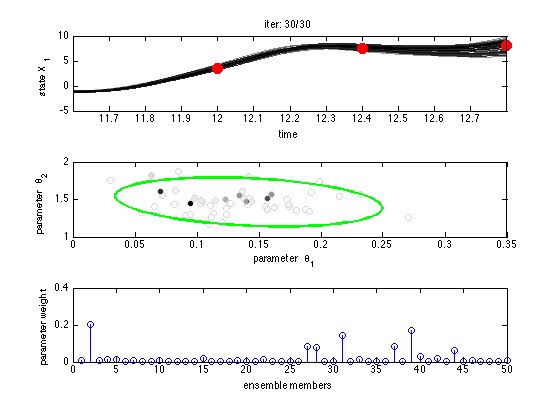
The figure shows iteratively the state evolution of each ensemble member for the first state variable X1, together with the observations. The forecast model lines are colored according to the forecast skill weight (upper panel). Two dimensional plot of the proposed parameters with their weights are shown with 95% probability ellipsoid of the proposal/prior covariance sig (center panel). The calculated relative weight for each members are shown (lower panel).

disp('... done')

... done

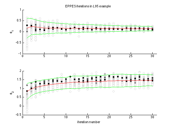
Plot the proposed points and their weights. For both of the parameters theta1 and theta2 the evolution of the EPPES method is shown. Iteration number is on the x axis and parameter value at y axis. Colouring shows the importance weights, red line is the evolution of the mean mu and green lines show plus minus 2 times the standard deviation from covariance matrix sig.

figure(2); clf
subplot(2,1,1)
eppeschainplot(parsall(:,:,1),weightsall, muall(:,1), sqrt(sigall(:,1,1)))
ylabel('\theta_1')
title('EPPES iterations in L95 example')
subplot(2,1,2)
eppeschainplot(parsall(:,:,2),weightsall, muall(:,2), sqrt(sigall(:,2,2)))
ylabel('\theta_2')
xlabel('iteration number')

Published with MATLAB® 7.12