EPPES example using linear model

This example demonstrates the ability of EPPES method to find the known true distribution in case of linear model.

We assume that observations are generated sequentially from y~N(theta,Sigma_{obs}) where the mean theta will be random, i.e. at each observation time window the value of theta is drawn from a hyper distribution theta~N(mu,Sigma). The parameters mu and Sigma are then estimated sequentially.

Laine, et al.: Ensemble prediction and parameter estimation system: the method, Q. J. R. Meteorol. Soc., 2011, doi:10.1002/qj.922.

npar = 3; % number of unknown parameters

True Sigma and mu.

trueSigma = covcond(10,ones(npar,1)) * 0.8
truemu = (1:npar)'
R = chol(trueSigma); % Cholesky factor of Sigma for random number generator

trueSigma =

      0.34182       0.2102      0.24799
       0.2102      0.36071      0.22909
      0.24799      0.22909      0.32292


truemu =

     1
     2
     3

Error std in observations.

sigeps = 0.8;

Initial guess/prior for mu and its accuracy.

mu = zeros(npar,1);
W  = eye(npar)*2^2;

Initial Sigma and its weight n.

Sig = eye(npar)*1.^2;  % this has to be big enough
n = 1; % how well we know Sig

nens  = 51; % ensemble size
nobs  = 10; % n:o of observations in one stage
nsimu = 200; % number of simulation stages

muall = zeros(nsimu,npar);
signorm = zeros(nsimu,1);
Wnorm = zeros(nsimu,1);

for isimu=1:nsimu
  theta =  mvnorr(1,truemu,trueSigma,R)'; % sample one theta from the true dist
  % we directly observe theta with error sigeps
  thetaobs = mvnorr(nobs,theta,eye(npar).*sigeps.^2);
  % posterior for theta when prior is prior N(mu,Sigma)
  Sigpost = inv(eye(npar)./sigeps.^2.*nobs+inv(Sig));
  mupost = Sigpost*(mean(thetaobs,1)'./sigeps.^2.*nobs+inv(Sig)*mu);
  % ensemble is drawn directly from the posterior
  thetaens = mvnorr(nens,mupost,Sigpost);
  % update hyper parameters according to the ensemble
  [mu,W,n,Sig] = eppesupd(thetaens,mu,W,n,Sig);

  % save
  muall(isimu,:) = mu';
  signorm(isimu) = norm(Sig-trueSigma);
  Wnorm(isimu)   = norm(W);

end

Now, mu should converge to truemu, Sig to trueSigma, W to zeros.

mu, Sig, W

mu =

       1.0402
       1.9858
       2.9456


Sig =

      0.34458      0.20097       0.2418
      0.20097      0.33381       0.2306
       0.2418       0.2306      0.33317


W =

    0.0017204   0.00093795    0.0012181
   0.00093795    0.0015914    0.0010834
    0.0012181    0.0010834     0.001753

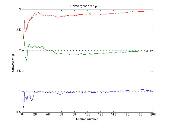
The first figure shows the convergence on mu to the true values given as horizontal lines.

figure(1); clf
plot(1:nsimu,muall)
for i=1:npar,hline(truemu(i));end
xlabel('iteration number'); ylabel('estimate of \mu')
title('Convergence for \mu ')

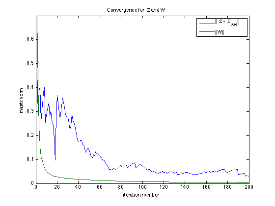
In the second figure, the norms of matrix W and difference Sigma-trueSigma are plotted with the iteration number.

figure(2); clf
plot(1:nsimu,signorm,1:nsimu,Wnorm)
title('Convergence for \Sigma and W')
xlabel('iteration number'); ylabel('matrix norm')
legend('||\Sigma - \Sigma_{true}||', '||W||')
ylim([0,0.7])

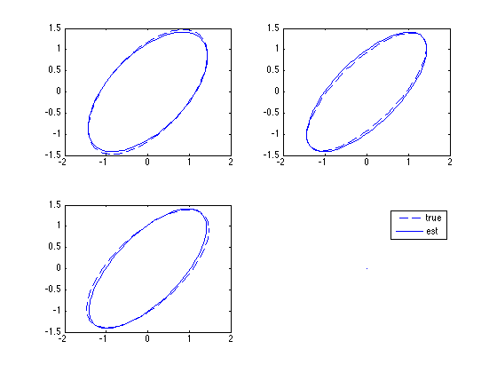
The last figure shows pair-wise 95% probability ellipsoids of the estimated Sigma and trueSigma at the last time window.

figure(3); clf
subplot(2,2,1);
ii=[1,2];
ellipse([0,0],trueSigma(ii,ii)*6,'--')
hold on
ellipse([0,0],Sig(ii,ii)*6,'-')
hold off
subplot(2,2,2);
ii=[1,3];
ellipse([0,0],trueSigma(ii,ii)*6,'--')
hold on
ellipse([0,0],Sig(ii,ii)*6,'-')
hold off
subplot(2,2,3);
ii=[2,3];
ellipse([0,0],trueSigma(ii,ii)*6,'--')
hold on
ellipse([0,0],Sig(ii,ii)*6,'-')
hold off
subplot(2,2,4);
plot(0,0,'--',0,0,'-b')
legend('true','est')
axis off

Published with MATLAB® 7.12