MCMC toolbox » Examples » Algae
Algae example
The example uses functions algaesys, algaefun and algaess.
We study the following system
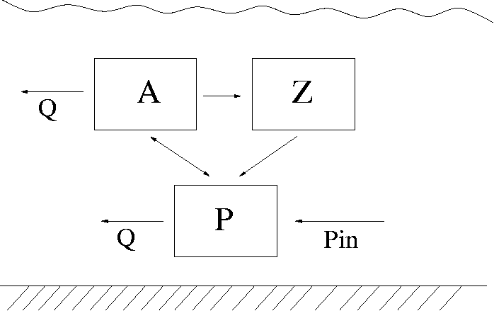
This is a simplified lake algae dynamics model. We consider phytoplankton A, zooplankton Z and nutrition P (eg. phosphorus) available for A in the water. The system is affected by the water outflow/inflow Q, incoming phosphorus load Pin and temperature T. It is described as a simple predator - pray dynamics between A and Z. The growth of A is limited by the availability of P and it depends on the water temperature T. The inflow/outflow Q affects both A and P, but not Z. We use the following equations:
dA/dt = (μ - ρa - Q/V - αZ) A
dZ/dt = αZA-ρz Z
dP/dt = -Q/V (P-Pin)
+ (ρa-μ)A+ρzZ
where the growth rate µ depends on both temperature T and phosphorus P
μ = μmaxθ(T-20)P/(k+P).
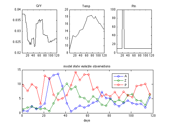
The data set is stored in algaedata.mat. First we load and plot the data.
clear model data params options
load algaedata.mat
figure
for i =1:3
  subplot(2,3,i)
  plot(data.xdata(:,1),data.xdata(:,i+1),'-k');
  title(data.xlabels(i+1)); xlim([1,120])
end
subplot(2,1,2)
plot(data.ydata(:,1),data.ydata(:,2:end),'o-');
title('model state variable observations');
legend(data.ylabels(2:end),0);
xlabel('days');
The model sum of squares in file algaess.m is given in the model structure.
model.ssfun = @algaess;
All parameters are constrained to be positive. The initial concentrations are also unknown and are treated as extra parameters.
params = {
    {'mumax', 0.5,  0}
    {'rhoa',  0.03, 0}
    {'rhoz',  0.1,  0}
    {'k',     10,   0}
    {'alpha', 0.02, 0}
    {'th',    1.14, 0, Inf, 1.14, 0.2}  % N(0.14, 0.2^2)1{th>0} prior
% initial values for the model states
    {'A0', 0.77, 0, Inf, 0.77, 2 }
    {'Z0', 1.3,  0, Inf, 1.3,  2 }
    {'P0', 10,   0, Inf, 10,   2 }
    };
We assume having at least some prior information on the repeatability of the observation and assign rather non informational prior for the residual variances of the observed states. The default prior distribution is sigma2 ~ invchisq(S20,N0), the inverse chi squared distribution (see for example Gelman et al.). The 3 components (A, Z, P) all have separate variances.
model.S20 = [1 1 2];
model.N0  = [4 4 4];
First generate an initial chain.
options.nsimu = 1000;
[results, chain, s2chain]= mcmcrun(model,data,params,options);
Sampling these parameters:
name   start [min,max] N(mu,s^2)
mumax: 0.5 [0,Inf] N(0,Inf)
rhoa: 0.03 [0,Inf] N(0,Inf)
rhoz: 0.1 [0,Inf] N(0,Inf)
k: 10 [0,Inf] N(0,Inf)
alpha: 0.02 [0,Inf] N(0,Inf)
th: 1.14 [0,Inf] N(1.14,0.2^2)
A0: 0.77 [0,Inf] N(0.77,2^2)
Z0: 1.3 [0,Inf] N(1.3,2^2)
P0: 10 [0,Inf] N(10,2^2)
Then re-run starting from the results of the previous run, this will take about 10 minutes.
options.nsimu = 5000;
[results, chain, s2chain] = mcmcrun(model,data,params,options, results);
Using values from the previous run
Sampling these parameters:
name   start [min,max] N(mu,s^2)
mumax: 0.557412 [0,Inf] N(0,Inf)
rhoa: 0.0793868 [0,Inf] N(0,Inf)
rhoz: 0.0996645 [0,Inf] N(0,Inf)
k: 9.74477 [0,Inf] N(0,Inf)
alpha: 0.025318 [0,Inf] N(0,Inf)
th: 1.02955 [0,Inf] N(1.14,0.2^2)
A0: 1.04487 [0,Inf] N(0.77,2^2)
Z0: 1.27712 [0,Inf] N(1.3,2^2)
P0: 10.6511 [0,Inf] N(10,2^2)
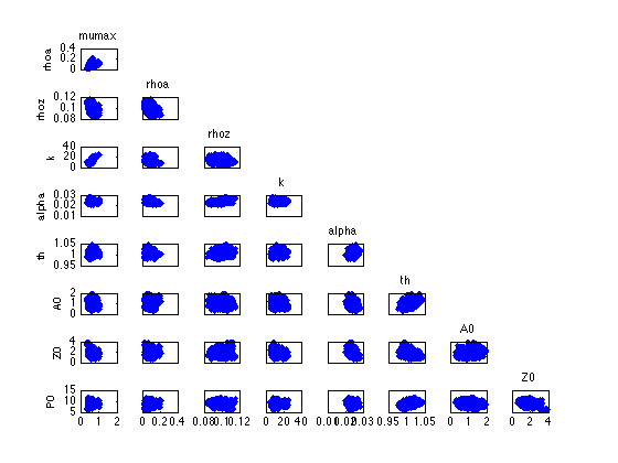
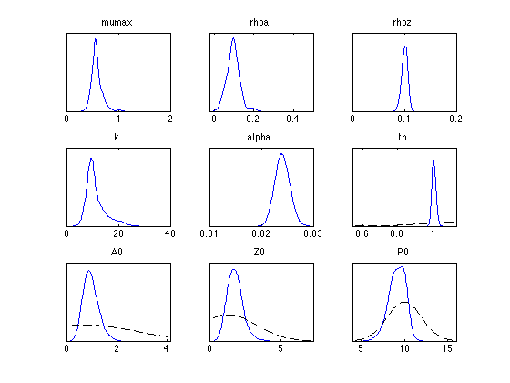
Chain plots should reveal that the chain has converged and we can use the results for estimation and predictive inference.
figure
mcmcplot(chain,[],results,'pairs');
figure
mcmcplot(chain,[],results,'denspanel',2);
Function chainstats calculates mean ans std from the chain and estimates the Monte Carlo error of the estimates. Number tau is the integrated autocorrelation time and geweke is a simple test for a null hypothesis that the chain has converged.
chainstats(chain,results)
MCMC statistics, nsimu = 5000

                 mean         std      MC_err         tau      geweke
---------------------------------------------------------------------
     mumax    0.58295     0.10072   0.0098423      59.983     0.88423
      rhoa   0.095294    0.032135   0.0030665      72.198     0.97093
      rhoz    0.10071    0.005465  0.00065503      124.01     0.92124
         k     11.192      3.6311     0.42752      92.865     0.68367
     alpha   0.024053   0.0013425  0.00011572      45.453      0.9596
        th     1.0069    0.010952   0.0010679      36.935     0.99297
        A0    0.96906     0.28734    0.030465      63.208     0.75098
        Z0     1.7996     0.52124    0.037832      30.294     0.87729
        P0     9.1803     0.91126      0.1118      147.28     0.82641
---------------------------------------------------------------------
In order to use the mcmcpred function we need function modelfun with input arguments given as modelfun(xdata,theta). We construct this as an anonymous function.
modelfun = @(d,th) algaefun(d(:,1),th,th(7:9),d);
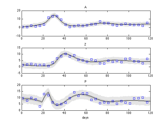
We sample 500 parameter realizations from chain and s2chain and calculate the predictive plots.
nsample = 500;
out = mcmcpred(results,chain,s2chain,data.xdata,modelfun,nsample);
figure
mcmcpredplot(out);
% add the 'y' observations to the plot
hold on
for i=1:3
  subplot(3,1,i)
  hold on
  plot(data.ydata(:,1),data.ydata(:,i+1),'s');
  ylabel(''); title(data.ylabels(i+1));
  hold off
end
xlabel('days');