RTO with BOD model

We use RTO to sample parameters in

$y = \theta_1(1-\exp(-\theta_2 x) + \epsilon \quad \epsilon\sim N(0,I\sigma^2)$

with data:

x = [1     3     5     7     9]';
y = [0.076 0.258 0.369 0.492 0.559]';
sig = 0.0136;               % known obs error (MSE from fit)
th = [0.9294  0.1040];      % LSQ fit with fixed data

model, jac, residual fcn

f = @(x,th) th(1)*(1-exp(-th(2)*x));
j = @(x,th) [1-exp(-th(2)*x) th(1)*x.*exp(-th(2)*x)]./sig;
resf = @(x,y,th) (y-f(x,th))/sig;

Initial MAP fit

th = lsqlevmar(@(th)resf(x,y,th), @(th)j(x,th), th);

save Q from qr decomposition of Jac at MAP

[Q0,~] = qr(j(x,th),0);

RTO sampling

nsimu = 5000;                   % no. of samples
thsim = zeros(nsimu,2);         % space for the chain
log_imp_wts=zeros(nsimu,1);     % space for log of weights
h = waitbar(0,'Doing RTO simulation...');
for i=1:nsimu
    % show progress
    if fix(i/100) == i/100;waitbar(i/nsimu,h);end

     % randomize ...
    ys = y+randn(size(y))*sig;
    % then optimize
    thsim(i,:) = lsqlevmar(@(th)Q0'*resf(x,ys,th),@(th)Q0'*j(x,th),th);
    % Jacobian and residuals at the new sample
    J = j(x,thsim(i,:));
    resid = resf(x,y,thsim(i,:));
    % compute correction factor, eqn (3.7) in the paper
    log_imp_wts(i) = rtodetlog(J,resid,Q0);
end
delete(h);

post-process and plot the results

acce = rtoaccept_log(log_imp_wts);    % Metropolis-Hastings
thsimfix = thsim(acce,:);

plotting

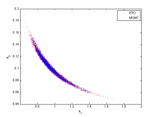
figure(1);clf
plot(thsimfix(:,1),thsimfix(:,2),'.r');
xlabel('\theta_1');ylabel('\theta_2');

MCMC sampling with DRAM. We simulate from the posterior distribution using MCMC with the DRAM algorithm.

J0 = j(x,th); qcov = inv(J0'*J0); % initial proposal covariance
[res,chain] = mcmcrun(struct('ssfun',@(th,d)sum(resf(x,y,th).^2)),...
                      [],...
                      {{'\theta_1',th(1)},{'\theta_2',th(2)}},...
                      struct('nsimu',nsimu,'qcov',qcov));

Sampling these parameters:
name   start [min,max] N(mu,s^2)
\theta_1: 0.929369 [-Inf,Inf] N(0,Inf)
\theta_2: 0.103995 [-Inf,Inf] N(0,Inf)

figure(1)
hold on
plot(chain(:,1),chain(:,2),'.b');
hold off
legend('RTO','MCMC')

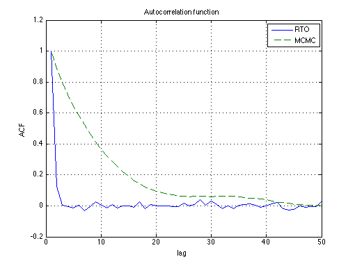
RTO simulation takes more time than MCMC, but from the autocorrelation function, we see that RTO is about 25 times more efficient that MCMC.

figure(2);clf
plot(1:50,acf(thsimfix(:,1),49),'-',1:50,acf(chain(:,1),49),'--')
grid; xlabel('lag'),ylabel('ACF'); title('Autocorrelation function');
legend('RTO','MCMC')