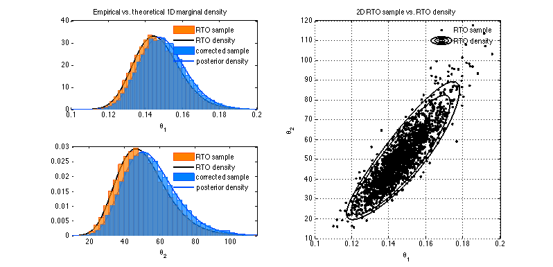
2D RTO example Monod model

We sample form the posterior of two parameters of the Monod model

$y = \theta_1 \frac{t}{\theta_2 + t} + \epsilon \quad \epsilon\sim N(0,I\sigma^2)$

given the data.

Data and initial values

x = [28,    55,    83,    110,   138,   225,   375]';
y = [0.053, 0.060, 0.112, 0.105, 0.099, 0.122, 0.125]';

th  = [0.15,50];           % initial theta
sig = 0.01;                % known observation error std

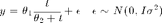
Model function, Jacobian, sum of squares

f = @(x,th) th(1).*x./(th(2) + x);
j = @(x,th) [x(:)./(th(2)+x(:)),-th(1).*x(:)./(th(2)+x(:)).^2];
ss = @(th,data) sum(((y-f(x,th))./sig).^2);

Initial fit and Q from qr decomposition of Jacobian at MAP

th = lsqlevmar(@(th)(y-f(x,th))/sig,@(th)j(x,th)/sig,th);
[Q0,~] = qr(j(x,th)/sig,0);

RTO sampling using Levenberg - Marquardt

nsimu = 20000;

thsim = zeros(nsimu,2); % rto sample
rtoc  = zeros(nsimu,1); % log correction factor
h = waitbar(0,'Doing RTO simulation...');
for i=1:nsimu
  if fix(i/500) == i/500;waitbar(i/nsimu,h);end
  ys = y+randn(size(y))*sig;   % randomize
  % then optimize
  thsim(i,:) = lsqlevmar(@(th)Q0'*(ys-f(x,th))/sig,@(th)Q0'*j(x,th)/sig,th);
  % log of the correction factor
  rtoc(i) = rtodetlog(j(x,thsim(i,:))/sig,(y-f(x,thsim(i,:)))./sig,Q0);
end
delete(h);

Resample to correct the sample

%thsimfix = logresample(thsim,2*rtoc);   % Importance sampling
thsimfix = thsim(rtoaccept_log(rtoc),:); % M-H sampling

Calculate the true posterior distribution over a mesh

ng = 100;
CC = zeros(ng); % correction factors
PP = zeros(ng); % true posterior
th1 = linspace(0.10,0.2,ng);
th2 = linspace(10,115,ng);
[TH1,TH2] = meshgrid(th1,th2);
cin = @(x,l1,u1, l2,u2)  sum( x(:,1)>l1 & x(:,1)<=u1 & x(:,2)>l2 & x(:,2)<=u2 );
d1 = th1(2)-th1(1); d2 = th2(2)-th2(1);
for ji=1:ng
  for ii=1:ng
    thi = [TH1(ii,ji),TH2(ii,ji)];
    CC(ii,ji) = exp(rtodetlog(j(x,thi)./sig,(y-f(x,thi))./sig,Q0));
    PP(ii,ji) = exp(-0.5*ss(thi,[]));
  end
end
RR = CC.*PP; RR = RR./sum(sum(RR)); % RTO distribution
PP = PP./sum(sum(PP));              % posterior distribution

Plotting

figure(1); clf
% theta_1 marginal
subplot(2,2,1)
nhist = 50;
h = histp(thsim(:,1),nhist);
set(h,'facecolor',[1 0.5 0],'edgecolor',[1 0.3 0]);
set(get(h,'Children'),'Facealpha',0.7);
hold on
h = plot(th1,sum(RR)./sum(sum(RR))/d1,'-','color',[0 0 0],'linewidth',2);
% posterior
h = histp(thsimfix(:,1),nhist);
set(h,'facecolor',[0 0.5 1],'edgecolor',[0 0.3 1]);
set(get(h,'Children'),'Facealpha',0.7);

plot(th1,sum(PP)./sum(sum(PP))/d1,'-','color',[0 0.3 1],'linewidth',2);
hl = legend('RTO sample','RTO density','corrected sample','posterior density');
set(hl,'box','off')
hold off
xlabel('\theta_1')
title('Empirical vs. theoretical 1D marginal density');
xlim(th1([1 end]));
% theta_2 marginal
subplot(2,2,3)
h = histp(thsim(:,2),nhist);
set(h,'facecolor',[1 0.5 0],'edgecolor',[1 0.3 0]);
set(get(h,'Children'),'Facealpha',0.7);
hold on
h = plot(th2,sum(RR')./sum(sum(RR'))/d2,'-','color',[0 0 0],'linewidth',2);
% posterior
h = histp(thsimfix(:,2),nhist);
set(h,'facecolor',[0 0.5 1],'edgecolor',[0 0.3 1]);
set(get(h,'Children'),'Facealpha',0.7);
plot(th2,sum(PP')./sum(sum(PP'))/d2,'-','color',[0 0.3 1],'linewidth',2);
hold off
hl = legend('RTO sample','RTO density','corrected sample','posterior density');
set(hl,'box','off')
xlabel('\theta_2')
xlim(th2([1 end]));
% 2D density
subplot(2,2,[2 4])
plot(thsim(1:10:end,1),thsim(1:10:end,2),'.k')
% contour limits
p1 = plims2dgrid(RR,[0.5 0.9 0.95]);
hold on
contour(th1,th2,RR,p1,'-k','linewidth',2);
hold off
xlim([0.1 0.2])
ylim([10 120])
grid
xlabel('\theta_1')
ylabel('\theta_2')
title('2D RTO sample vs. RTO density')
hl = legend('RTO sample','RTO density');
set(hl,'box','off')