Figure 1
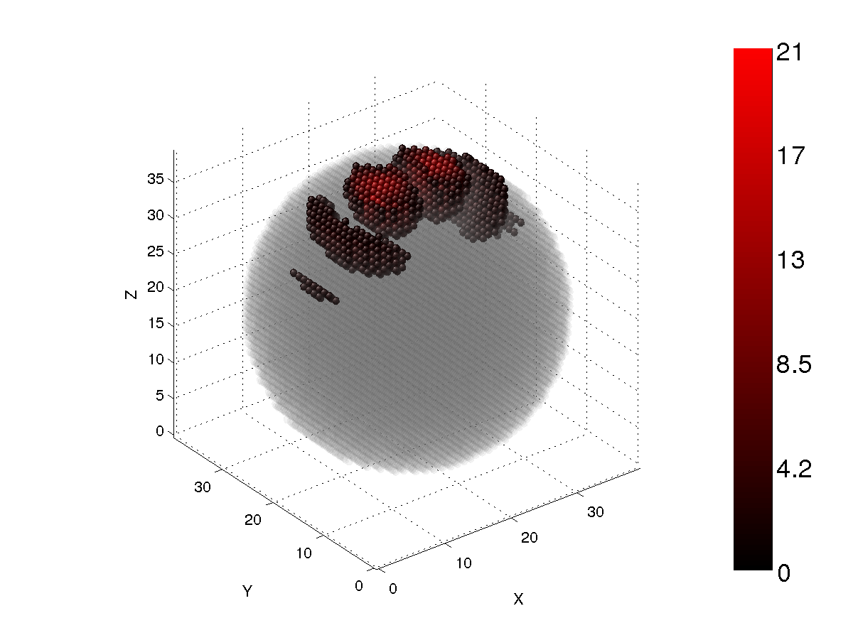
Figure 2
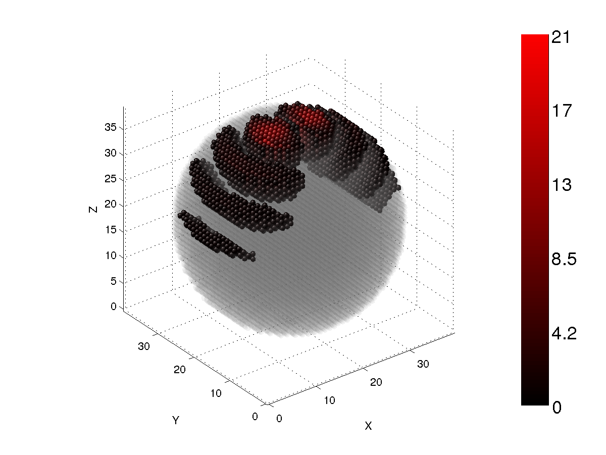
Figure 3
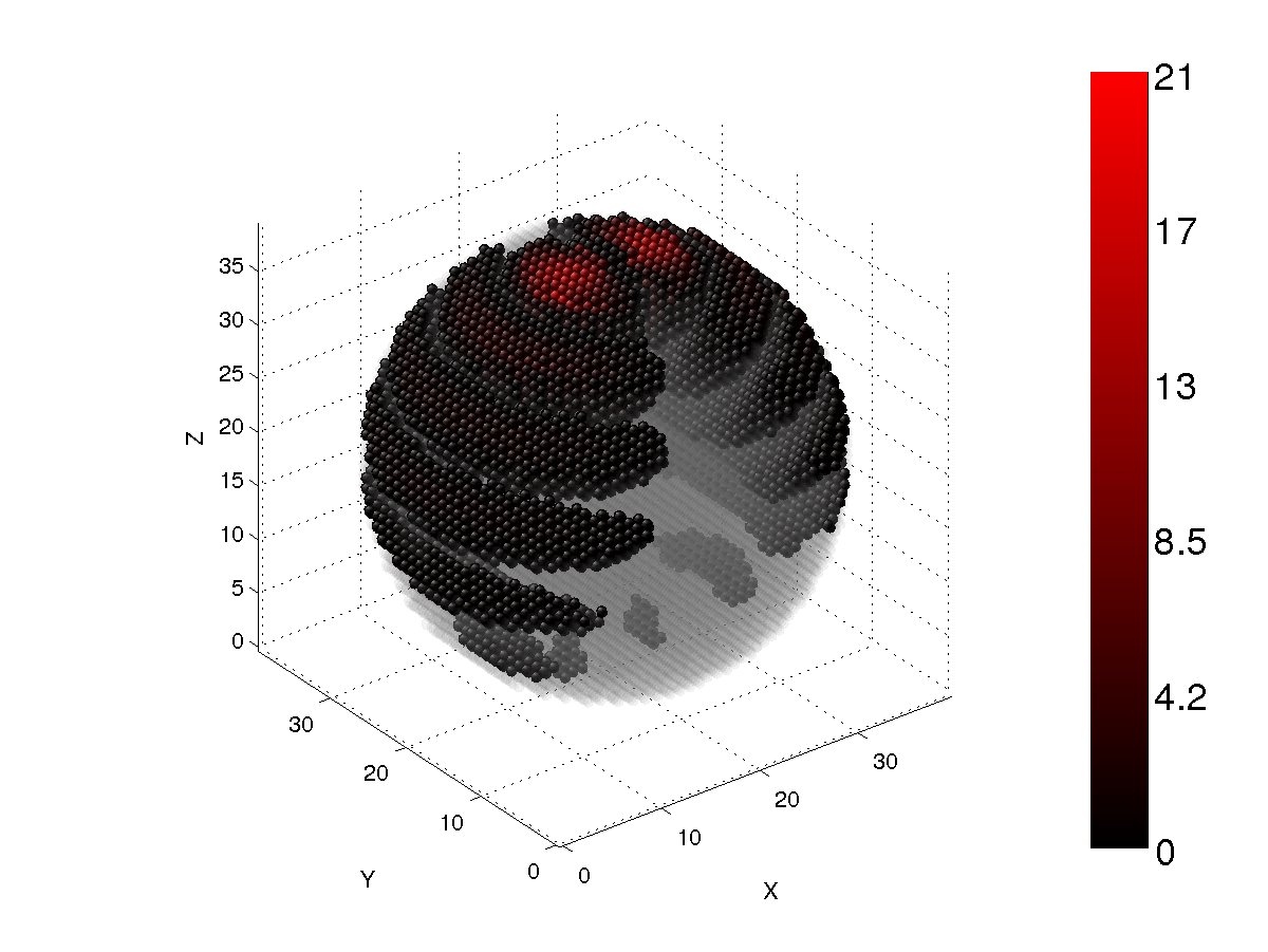
Figure 4
Particles with sizes small compared to the wavelength, both outside (x=2πa/λ<<1, &lambda is wavelength, a is radius) and inside (|m|x=<<1) the particle can be modeled as a single radiating dipole (Rayleigh scattering). Single dipoles show a typical bell-shaped curve for the degree of linear polarization, which is positive for all scattering angles. When the size of the particle increases, it can no longer be approximated with a single dipole, but requires many dipoles. A system of dipoles organized to a regular grid can be modeled with, for example, the discrete-dipole approximation (DDA). Dipoles that are near each other, produce interference between the electromagnetic waves that scatter from them. When computing the far field from these waves, the degree of linear polarization can have non-Rayleigh-type features, like negative polarization, at certain scattering angles. Wavelength-scale particles are large enough, that usually many dipoles are required to compute the scattering in the far field. They are also small enough, that interference between different parts of the particle play an important role. Scattering from large particles (x>>1) can be moleded with the geometric optics approximation (GOA), which treats the plane waves as rays, which do not interfere with each other.
The role of interference between the dipoles inside wavelength-scale particles can be studied using DDA by first computing the induced field at each dipole site, then modifying the induced fields, and finally recomputing the far field from the modified internal field. This kind of modification is of course artificial and cannot be observed or measured in reality. In principle, this could be done, if each dipole could be replaced with an antenna in an microwave analog experiment, and controlled independently from each other.
Normally, when observing single particles in remote sensing experiments, the measured value is an integrated quantity from all parts of the particle. For certain incident plane wave and scattering angle, one value is measured. In DDA, the far field is an integrated sum of the induced fields from all dipoles. Instead of integrating across the whole particle, a study of partial integration can be made. These partial integration maps provide information of the interaction between the dipoles, and shed light to the role of interference inside the modeled particles.
Polarization of the incident plane wave can be used to study interference effects inside particles. Polarization is usually described by the Stokes vector with four observable elements, and the scattering by the Mueller matrix. The Mueller matrix of the particle depends on many things, like the shape, size, refractive index, and orientation of the particle. It transforms the incident Stokes vector to the scattered Stokes vector, which, in addition to the properties of the particle, also depends on the incident polarization state of the wave and its incident propagation direction (wave vector). This is valid in the laboratory reference frame. In the particle reference frame, the coordinate system changes according to the orientation of the particle relative to the laboratory reference frame. In the scattering reference frame, the coordinate system changes according to the incident wave vector relative to the laboratory reference frame.
In this study, the laboratory reference frame is assumed to be cartesian, the particle is oriented in a fixed direction, the incident plane wave is propagating to the direction of positive Z-axis, and the incident electric field is either X- or Y-polarized. In this reference frame, the internal field is also cartesian, with the Z-component parallel to the incident wave vector, and the X- and Y- components parallel to the incident polarization. The former is from now on called the longitudinal component and the latter as transverse components of the internal electric field. The scattering plane (plane defined by the incident and scattered wave vectors) is chosen to be the XZ-plane, which means that the X-polarized incident wave is parallel to the plane, and Y-polarized incident wave is perpendicular to the plane. The observer is always in the scattering plane measuring both the parallel and perpendicular components of the scattered wave. The degree of linear polarization for unpolarized incident wave is defined as P = I_perp - I_par / I_perp + I_par. Since natural light is highly unpolarized, the final result is averaged over two incident, mutually perpendicular polarizations (X and Y).
To identify the dipoles that have the most contribution to the longitudinal component, defined as 'core dipoles', the dipoles are first sorted based on their longitudinal energy density from the brightest to the darkest. Then a cutoff value is chosen, which defines the ratio of the total energy density of the most brightest core dipoles to the total energy density of all dipoles. Dipoles that have brightness less than defined by the cutoff are called non-core dipoles.
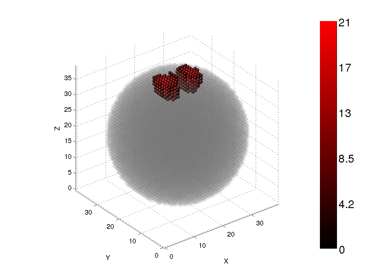
Figs. 1-4 show the longitudinal energy density of a spherical particle with the size parameter x=7.9 and the refractive index m=1.5+i0.01. The cutoff values are 30%, 50%, 70%, and 90%. The incident wave is X-polarized. As can be seen, the internal field is highly concentrated at the forward part of the particle. There are two dipole regions that are symmetric with respect to the central plane of the particle for the 30% cutoff case. The relative number of core dipoles is only about 1%, which indicates very strong focusing of the internal electric field. When the cutoff value is increased (Figs. 2-4), the number of core dipoles increases, but most are still concentrated at the forward part of the particle. At 90% cutoff, the relative number of core dipoles is only about 36% for spheres.
Figure 1
Figure 2
Figure 3
Figure 4
Figs. 5-8 show the same as Figs. 1-4, but for a Gaussian-random-sphere particle with circumscribing size parameter x=12 and the refractive index m=1.5+i0.01.
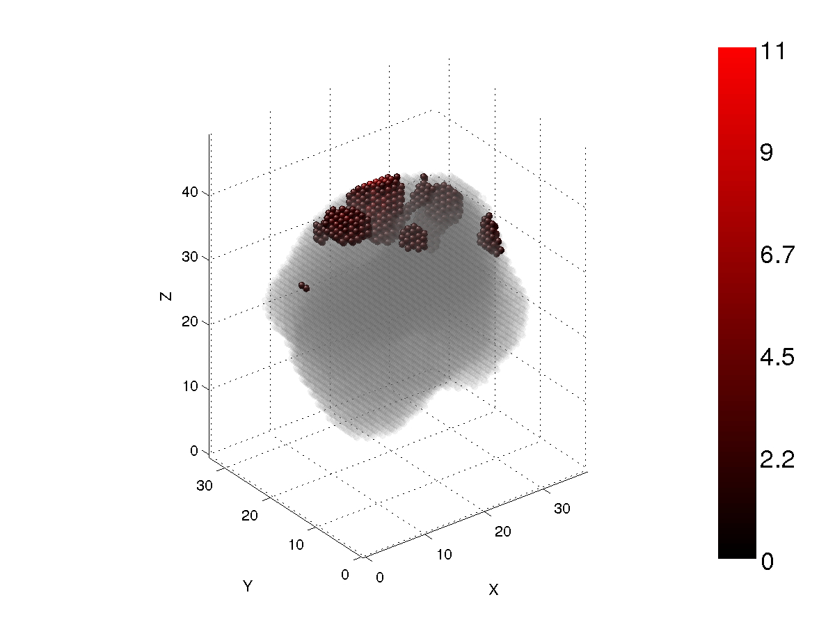
Figure 5
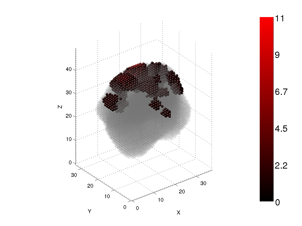
Figure 6
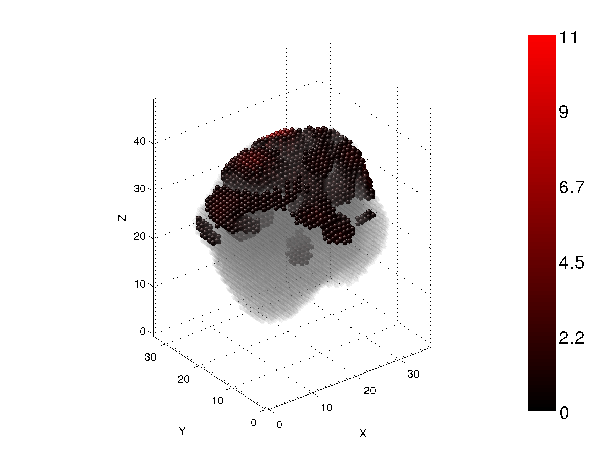
Figure 7
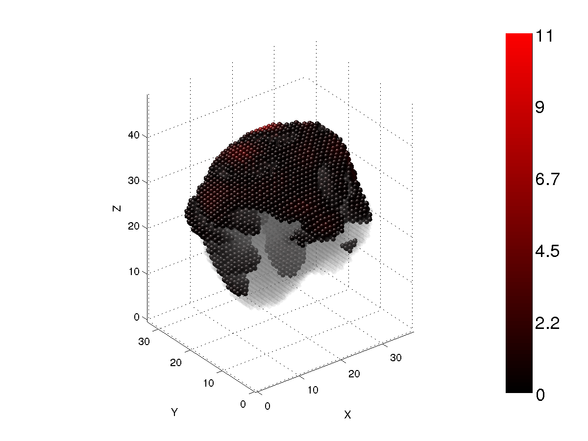
Figure 8
Figs. 9-12 show the same as Figs. 1-4, but for a agglomerated-debris particle with circumscribing size parameter x=12 and the refractive index m=1.5+i0.01.
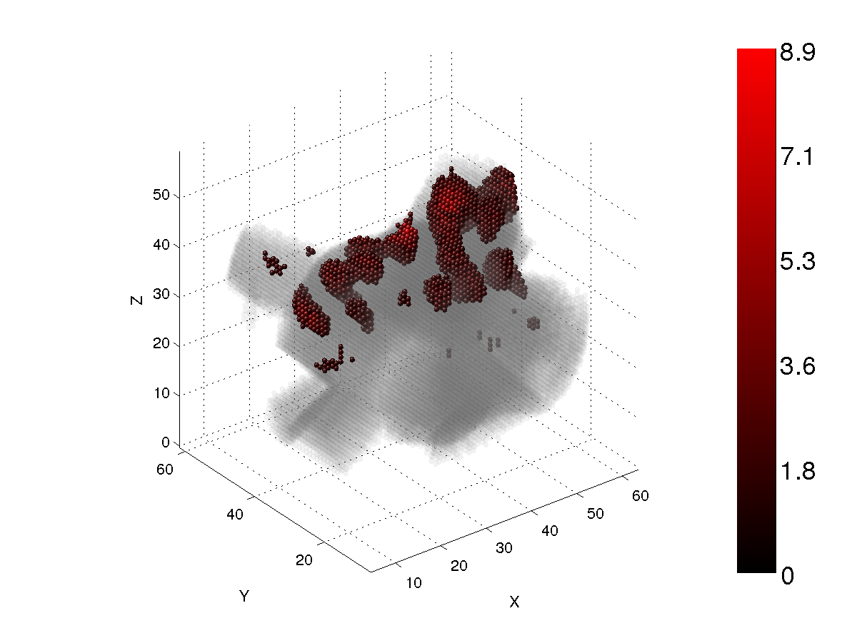
Figure 9
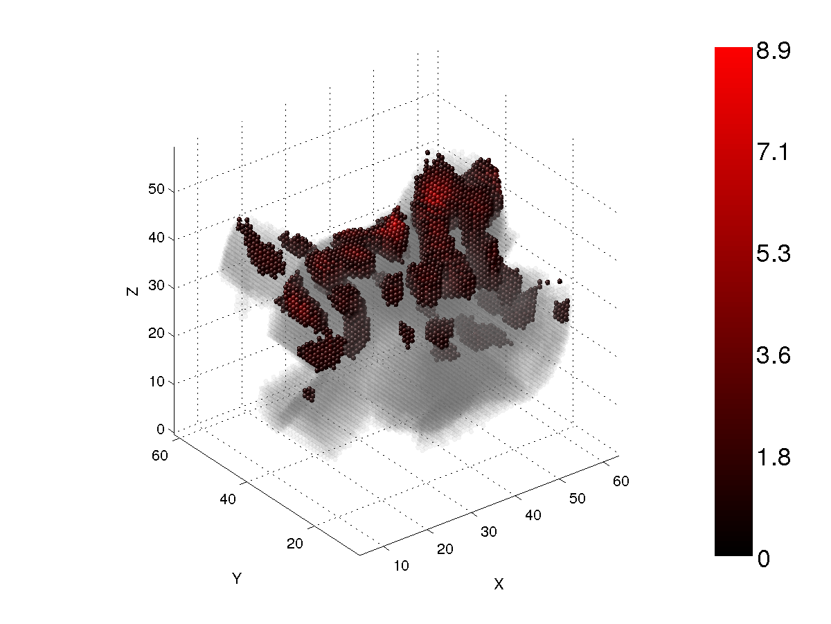
Figure 10
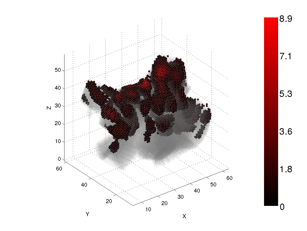
Figure 11
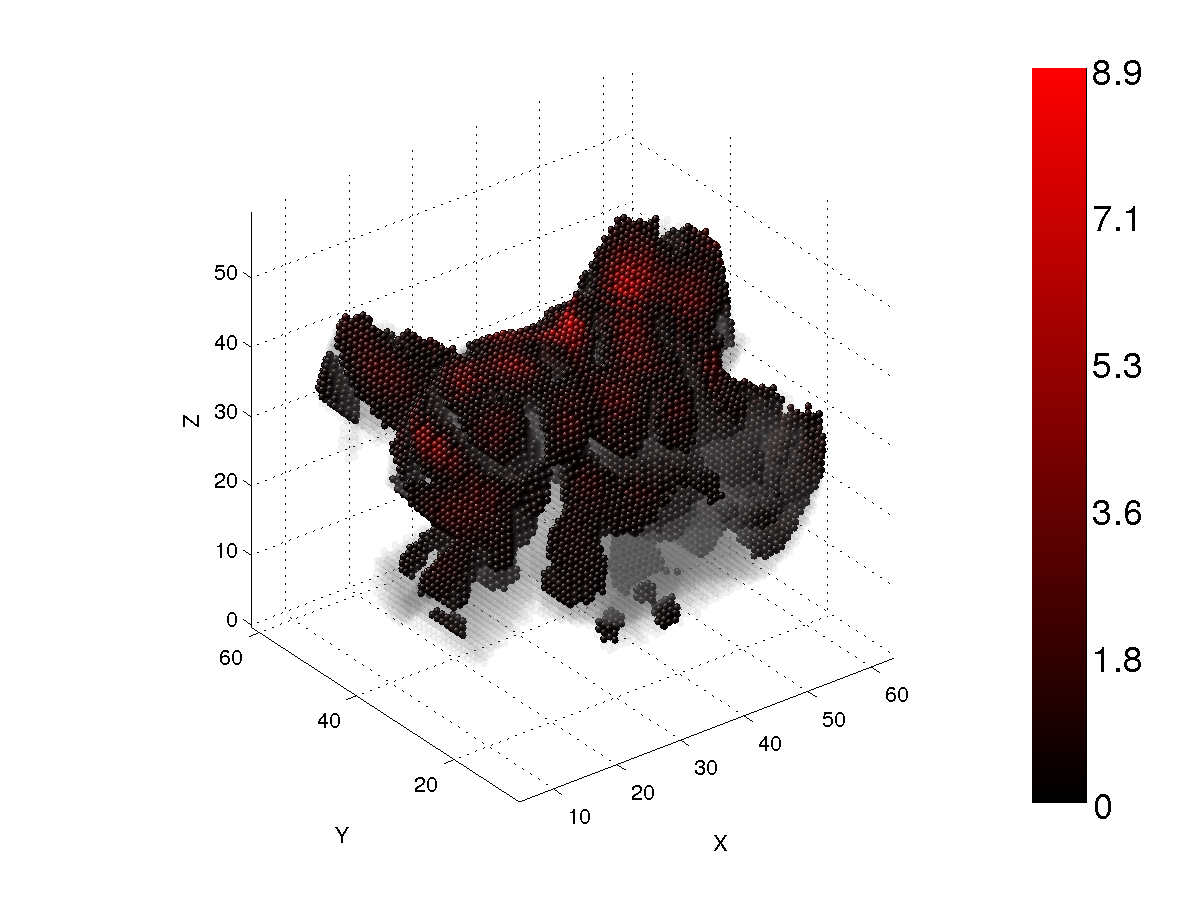
Figure 12
To study the role of interference inside wavelength-scale particles, we use a partial integration scheme for the internal field, when computing the far-field scattering characteristics. We first compute the total electric field from columns of dipoles that are projected to a tangent plane. These projected fields are computed coherently among the columns, which each represent one point in the plane. We then compute the far-field scattering components separately for each point in the projected plane as a function of the scattering angle. We also integrate further over the two transverse directions, X- and Z-axes for 90 deg scattering angle, to reveal phase differences between the maxima in the projected plane. It should be noted that this procedure is purely a mathematical tool and not something that could be observed or measured.
In Fig. 13, we show the contributions of the internal longitudinal components on the far-field scattering intensities at 90 deg scattering angle. The incident field is polarized parallel to the scattering plane. There is a very bright area at the forward part of the particle, which is caused by focusing of the incident wave. For spherical particles, it is symmetric. The whole region is in phase, which can be seen as enhancement in the graph above the figure (integration over X- and Z-directions). This will produce constructive interference between the core regions.
In Fig. 14, we show the same as in Fig. 13, but the incident field is polarized perpendicular to the scattering plane. There are two weaker core regions that have opposite phases, which can be seen as cancellation in the graph above the figure (integration over X- and Z-directions). This will produce destructive interference between the core regions. The contribution from the core regions is significanlty dampened for the perpendicular incident field than for the parallel incident field. This means that interference in the longitudinal component is the main reason for the non-Rayleigh-type polarization at intermediate scattering angles.
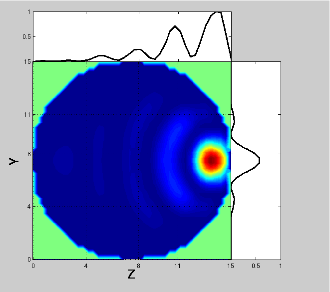
Figure 13
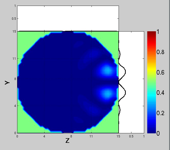
Figure 14
In Figs. 15-16, we show the same as in Figs. 13-14, but for the Gaussian-random-sphere particle. The same conclusions hold as for the spherical particles.
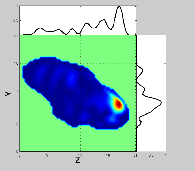
Figure 15
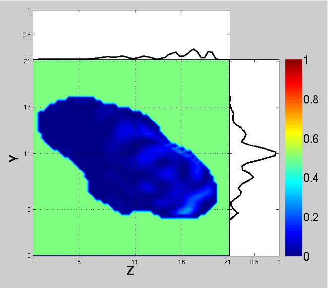
Figure 16
In Figs. 17-18, we show the same as in Figs. 13-14, but for the agglomerated-debris particle. The same conclusions hold as for the spherical particles.
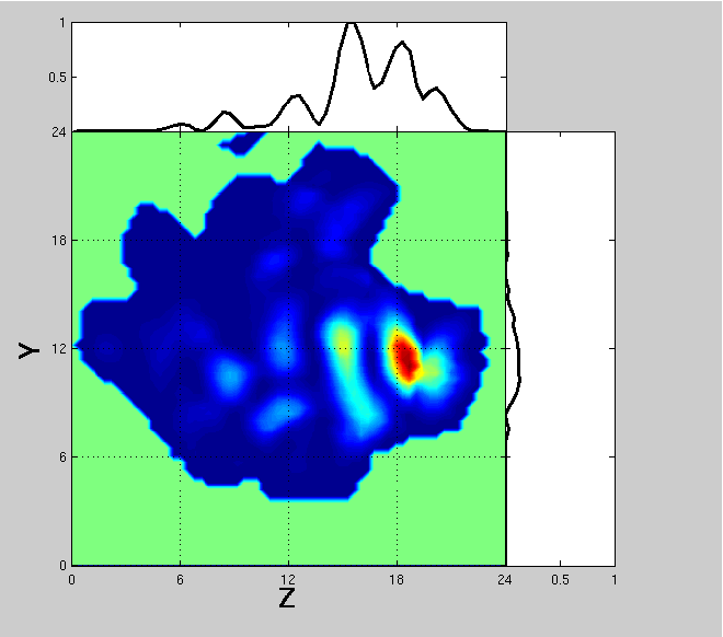
Figure 17
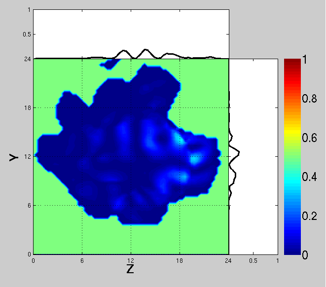
Figure 18
In Figs. 19-20, the interference mechanism is presented as a diagram for the parallel (Fig. 19) and perpendicular (Fig. 20) incident field.
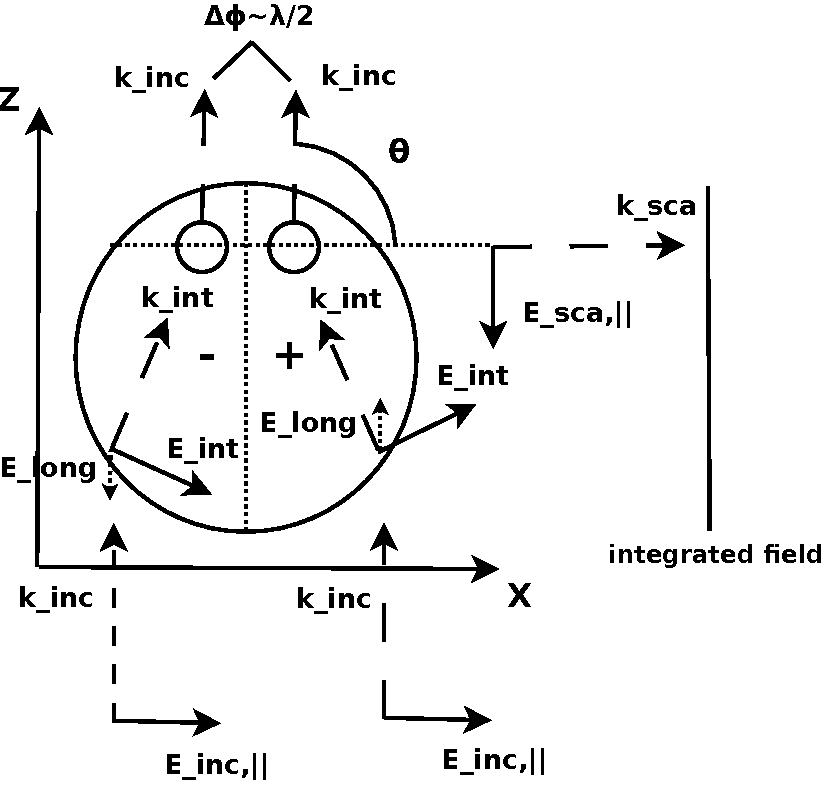
Figure 19
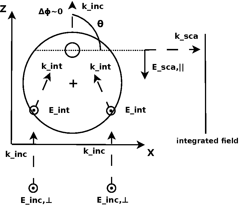
Figure 20
Here are the links to movie files showing the cases in Figs. 13-18 as a function of the scattering angle.