RTO - Randomize-then-optimize

The web page is accompanying a paper by J. M. Bardsley, A. Solonen, H. Haario, M. Laine: Randomize-then-Optimize: A Method for Sampling from Posterior Distributions in Nonlinear Inverse Problems in SIAM journal on Scientific Computing, 36(4), 2014, doi: 10.1137/140964023. Here is the abstract:

High dimensional inverse problems present a challenge for Markov Chain Monte Carlo (MCMC) type sampling schemes. Typically, they rely on finding an efficient proposal distribution, which can be difficult for large-scale problems, even with adaptive approaches. Moreover, the autocorrelations of the samples typically increase with dimension, which leads to the need for long sample chains. We present an alternative method for sampling from posterior distributions in nonlinear inverse problems, when the measurement error and prior are both Gaussian. The approach computes a candidate sample by solving a stochastic optimization problem. In the linear case, these samples are directly from the posterior density, but this is not so in the nonlinear case. We derive the form of the sample density in the nonlinear case, and then show how to use it within both a Metropolis-Hastings and importance sampling framework to obtain samples from the posterior distribution of the parameters. We demonstrate, with various small- and medium-scale problems, that RTO can be efficient compared to standard adaptive MCMC algorithms.

Briefly, RTO is a method for sampling from the posterior distribution of model parameters in nonlinear inverse problems of form

\begin{equation*} y = f(x;\theta) + \epsilon, \text{ where } \epsilon \sim N(0,\Sigma), \end{equation*}

with known error covariance matrix \(\Sigma\). A basic and well known idea is to study the sensitivity of parameter values by resampling the observations \(y^{*} = y + \xi^{*}\), where \(\xi^{*}\) is sampled from \(N(0,\Sigma)\), and then repeatedly solving the least squares optimization problem using the new data \(y^*\) to obtain a new solution \(\theta^*\). This is a form of parametric bootstrap method. However, the distribution of the sample of parameter values obtained is not known in general, even in the Gaussian case.

If we knew that this produces samples from a distribution \(c(\theta)p(\theta|y)\), where \(p(\theta|y)\) is the posterior distribution of interest and \(c(\theta)\) is a known correction factor that can depend on \(\theta\), then we could use importance sampling or Metropolis-Hastings acceptance step to correct the sample. For the direct randomization approach the distribution is not known. But, if we modify the problem a little, we are able to make sampling procedure where we can find out the actual sampling distribution, calculate \(c(\theta)\), and correct the distribution to produce a sample from the posterior distribution of \(\theta\). This is the RTO method described in the paper.

Instead of the optimization problem $$\mathop{\mathrm{argmin}}_{\theta^*}||y^* - f(x,\theta^*)||^2$$ we solve a slightly modified problem $$\mathop{\mathrm{argmin}}_{\theta^*}||Q_0' (y^* - f(x,\theta^*))||^2,$$ where \(Q_0\) is the Q matrix from thin QR decomposition of the Jacobian matrix at the original map estimate of θ. Here, we have assumed that the error covariance is an unit matrix, i.e. \(\Sigma = I\), achieved by suitable pre-whitening of the problem. For this problem, we can show that the correction factor is $$c(\theta^*) = |Q_0'J(\theta^*))| + \frac12(||r(\theta^*)||^2-||Q_0'r(\theta^*)||^2),$$ where \(r(\theta^*) = y - f(x;\theta^*)\) is the residual calculated using the RTO sample point against the original data. A logarithm of this factor is calculated by function rtodetlog.m in the Matlab code provided here. Please refer to the paper for more details and the assumptions needed.

• rto.zip (updated 2014-08-01) RTO Matlab files and examples.
• mcmcstat.zip the Matlab MCMC Toolbox, needed in the examples.

The file rto.zip contains Matlab code for RTO calculations, some routines for plotting the results and some example code.

The code is provided for demonstration purposes, it is distributed under a MIT License and comes with no warranty. Please read the RTO paper and the source code provided for details of the algorithm. Question and suggestions are welcome. If you find the code useful, you should cite the RTO paper in your research articles.

The example Matlab codes are in rto.zip given above. The files do not depend on any other Matlab toolbox than the MCMC toolbox. So far, we provide two 2 dimensional parameter estimation examples. RTO sampling is intended for high dimensional problems, however. In the paper we demonstrate RTO for 200 dimensional estimation problem originating from satellite remote sensing of atmospheric constituent profiles.

Monod 2D example

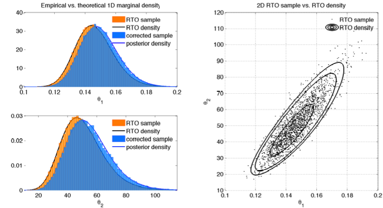
Monod example samples 2D parameter using RTO and compares the sample to the theoretical RTO distribution, then corrects the sample and compares it to the posterior distribution. The theoretical distributions are calculated by 2D numerical integration. File rtoexample_monod.m in rto.zip.

BOD 2D example

BOD example is another 2D parameter estimation example. Now we compare the efficiency of RTO to that of MCMC using the DRAM method. File rtoexample_bod.m in rto.zip.

J. M. Bardsley, A. Solonen, H. Haario, M. Laine: Randomize-then-Optimize: A Method for Sampling from Posterior Distributions in Nonlinear Inverse Problems, 36(4), pages A1895–A1910, 2014. doi: 10.1137/140964023.

---